2.3. Setup the Workflow
The left panel contains a tree view that displays the workflow, parameters and KPIs and optimizer. Clicking on any item in the tree brings up fields and buttons in the right panel for setting the selected attribute.
Below we will create one execution layer with two Gaussian data sources. Each data source describes a two-dimensional Gaussian on the x-y plane.
With a negative peak amplitude (a peak) the Gaussian forms a minima in xy-parameter space. With the amplitudes of two such Gaussians as the criteria/KPIs, the Pareto front stretches between their two minima. We will find this front using an MCO built on top of the Nevergrad gradient-free optimization library. This MCO is provided by a dedicated plugin.
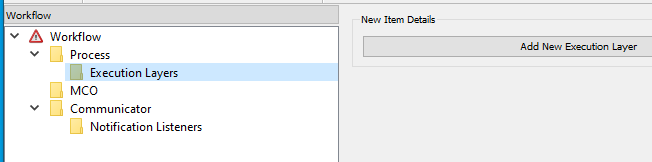
2.3.1. Create an Execution Layer
Select the Execution Layers tree-item and press the Add New Execution Layer
button. A tree-item, Layer 0, appears under Execution Layers.
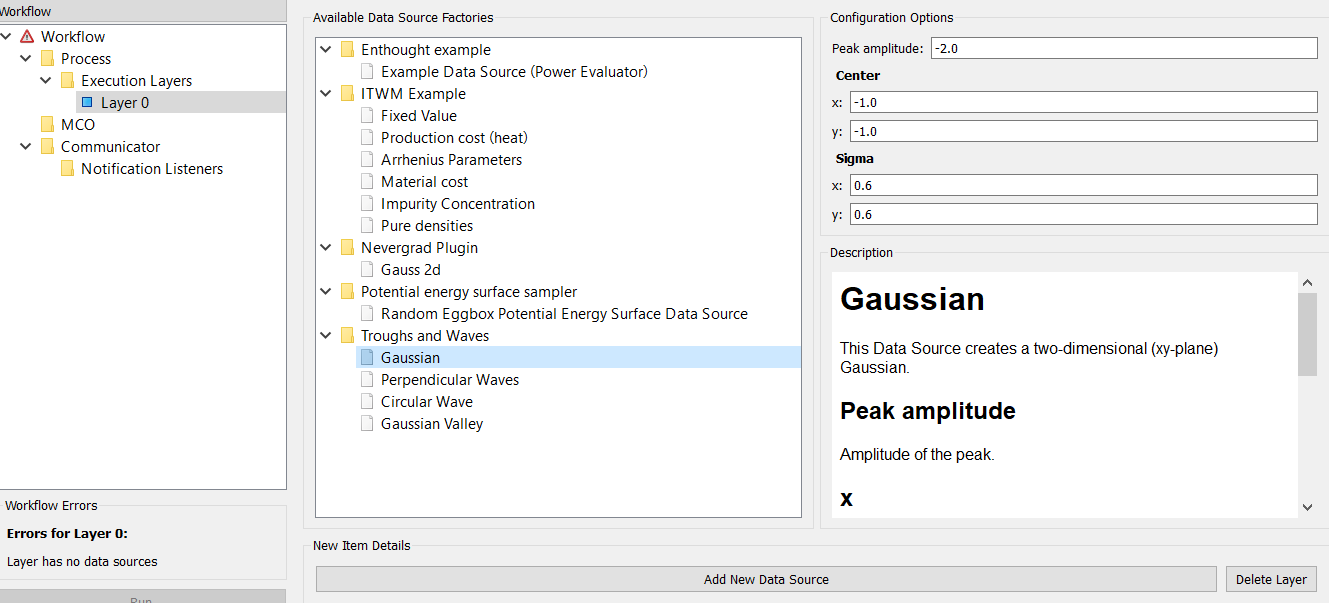
2.3.2. Add a Data Source
Selecting the Layer 0 tree-item brings up two panels at the right:
Available Data Source Factories- A tree-list of all the available data sources, arranged by the plugin that has contributed them.
Configuration Options/Description- A description of the data source.
Select one the Gaussian data sources contributed by the Troughs and Waves plugin
and press the Add New Data Source button to add it to the execution layer.
The data source is added as a tree-item under Layer 0. Selecting this item
brings up four panels at the right:
Input variables- The list of inputs.
Output variables- The list of outputs.
Selected parameter description- The description of the selected input/output.
- A
listof constants that will not be optimized.
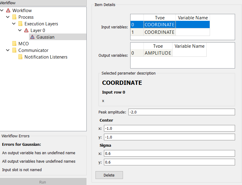
The Variable Name fields of the Input variables and output variables are used to
connect data sources in different execution layers. Any output-input pair that you want to
connect as an edge, should be given the same Variable Name.
Otherwise you can enter anything you like: it is easiest to use
the name that appears in Selected parameter description. This is
what we will do for the Gaussian data source, as we are not
connecting it to another data source (both Gaussian data sources will be in
the same execution layer).
Add a second Gaussian data source to the same execution layer. The list of constants for the Gaussian data source are:
- the peak amplitude
- position of the peak (
Centerx and y coordinates) - width of the peak (standard deviation or
Sigmaalong the x and y axis)
Center the Gaussians at (-1, 1) and (1, 1) with amplitudes of -2 and -1, respectively. The first Gaussian is then global minimum whereas the second is a local minimum.
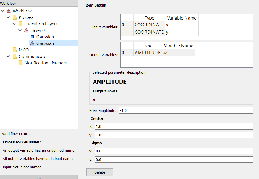
Their Input variable names should be the same (e.g. x and y), so that they
refer to the same x and y parameters.
Their Output variable names (their amplitudes) should be different (e.g. a1 and a2),
so that they are recognised as separate KPIs.
2.3.3. Select an Optimizer
Selecting the MCO tree-item brings up two panels at the right:
Available MCO Factories- A tree-list of all the available optimizers, arranged by the plugin that has contributed them. Note that not all of these will be multi-criterion optimizers.
Configuration Options/Description- A description of the selected optimizer.
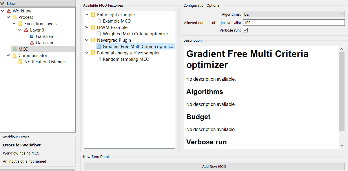
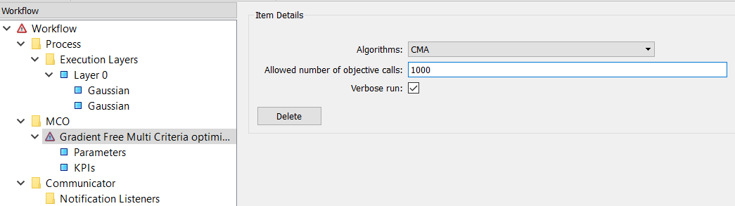
Select an optimizer and press the Add New MCO button. The optimizer is added as a tree-item
under MCO. Selecting this item brings up a single panel to the right:
Item Details- Certain parameters that control how the optimizer works.
Select CMA for the algorithm and set 1000 for Allowed number of objective calls.
2.3.4. Select the Parameters
Under the optimizer are two further tree-items for setting the parameters and KPIs.
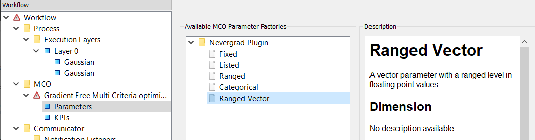
Selecting the Parameters tree-item brings up two panels at the right:
Available MCO Parameter Factories- A tree-list of all the available parameters for the optimizer.
Description- The description of the selected parameter.
When we specify a “parameter”, as well as selecting a data source input we must also tell the optimizer how to treat that input: its parameterization. Is the parameter:
- fixed (i.e. a constant)?
- continuous, with a lower and upper bound?
- categorical, a member of an ordered or unordered set?
Certain optimizers can only handle certain parameterizations. For instance, gradient-based optimizers can only handle continuous parameters, not categorical (which don’t have a gradient). The Nevergrad optimizer can handle all types, but for now we will only use continuous (‘Ranged’).
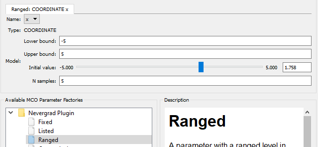
Select the Ranged item and press the New Parameter button. A new
panel appears at the top-right. This will contain a tab for each
parameter added. A Ranged parameter tab has the following fields:
Name- A drop-down list of data source inputs. Select the input “x”, the x coordinate.
Lower bound- Set the lower bound to -5.
Upper bound- Set the lower bound to 5.
Initial value- Slide this to anything (it doesn’t matter to the Nevergrad optimizer).
N samples- This has no meaning and can be ignored.
Add another Ranged parameter for the y coordinate and set the same
bounds and initial value.
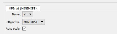
2.3.5. Select the KPIs
Selecting the KPIs tree-item brings up a New KPI button. Pressing
this button brings up a tabbed pane, one tab for each KPI added
with the following fields:
Name- A drop-down list of data-source outputs. Select the output “a1”, the amplitude of the first Gaussian data source.
Objective- Choose whether to minimize or maximize the KPI. With maximize chosen, the KPIs are simply negated during optimization. In our case choose minimize as the Gaussians have negative peak amplitude. If you make the Gaussian peaks positive and then choose maximize: this will give you the same results.
Auto scale- This is used by some of the optimizers to scale the KPIs so that they have comparable amplitudes. The Nevergrad optimizer does not scale, so ignore this.
Add a KPI for the second Gaussian (“a2”) in the same manner.