1.1. Optimization
Optimization is the task of finding the set of parameters of a process that are “best” (optimal) in terms of a set of criteria, objectives or key performance indicators. For instance a soap factory might be looking for the optimal ratio of different fats and hydrolysis temperature (the inputs) that produce a soap that has the best smell, the most suds and is cheap (the criteria/objectives)/KPIs.
Key Performance Indicator (KPI)
A performance indicator that has a target value and is declared to be of importance to the company. A KPI can be a combination of one or more performance indicators, e.g. in objective functions. A performance indicator can be declared to be a key performance indicator if there is a target value related to it.
Traditionally manufacturers have optimized their process at the R&D lab bench, before scaling-up to the plant or factory. Optimization is guided, like any good experiment, by a mixture of theoretical knowledge, expert intuition and brute-force: just trying as many parameter combinations as possible in the time allowed. This is of course all very costly in terms of time and money, so for a long time manufacturers have employed computational models of their process.
Computational models are quick and cheap (at least relative to the bench), can themselves use past experimental data and can simulate the at-scale process rather then a miniature version. They will never supplant the bench, but they can reduce the leg-work. In industries such as aerospace, computer models have been a vital element of R&D for decades. In the materials and chemical industry, modelling is being driven by the increasing need for diverse, exotic and tailored materials. How can one optimize a computer model of such a material’s manufacture? Formally one can describe the process to be optimized as a mathematical function. The function has inputs (parameters) and outputs (objectives or criteria). The function itself is sometimes called the objective function. The value of each input is an axis in parameter space. Each point in parameter space is associated with a set of output/objective values. With two parameters (x and y, say), a two-dimensional parameter space, the output (z) can be visualised as a surface on the xy-plane with z as the height of the surface. For objective functions with more than two inputs, the output surface is a hypersurface in a multi-dimensional parameter space.
The definition of what is “optimal” depends on whether the objective function (process) has a single output or multiple outputs (criterion).
1.1.1. Single-criterion optimization
A function with a single output is a scalar function. The maxima and minima and are valley-bottoms and peaks of the output’s surface, respectively. The global minimum/maximum is the lowest/ highest valley-bottom/peak, respectively. Other valley-bottoms/peaks are local minima/maxima. The task of optimization is then to find at best the global minimum/maximum or at least a local minima/maxima.
1.1.2. Multi-criterion optimization
If the objective function has more than one output, there are multiple surfaces, each with its own minima and maxima. At any point in parameter space, either:
- The slopes of the output surfaces all point in the same direction (all up or all down).
- One can always move away from that point and either increase all the outputs/criteria simultaneously or decrease all of them.
- The slopes of the output surfaces point in opposite directions.
- Making a move always increases at least one output whilst decreasing at least one of the others. These conditions are known as Pareto dominated and Pareto efficient, respectively, after the Italian engineer and economist Vilfredo Pareto. He said that the optimal situation is when we cannot improve all outcomes simultaneously - that is a Pareto efficient point. The task of optimization is to find the set of Pareto efficient points. These points often form along a line through parameter space, the Pareto front.
Typically an industrial process will have multiple optimization criteria. Thus such algorithms are vitally important but have rarely been used through a lack of expertise and commonly available computational libraries or softwares that implement them.
1.1.3. Optimizing a Directed Graph
Many processes can be divided up into granular, near-self-contained sub-processes, with the output of one feeding into the input of another. For instance a soap production line might be divided up into the melting of the fat, the hydrolysis chamber, the mold cooling, milling and packing. It is often helpful to reproduce these divisions when simulating a process with a computer. Each sub-process is a function with inputs and outputs which feed one into another. The functions might include molecular-dynamics or computational fluid dynamics simulations, interpolation of experimental data or economic cost-price calculations. The inputs and outputs might include concentrations of particular chemicals, physical parameters such as temperature and pressure, price and quality of materials or manufacture time.
There are many names for a set of connected sub-processes. The pipeline is common in computer science, but has a clear industrial origin - reaction vessels (sub-processes) connected by pipes. Another name is a workflow, with the clear flavor of the office. A mathematician would define it as a directed graph, with the sub-processes as nodes and the connections as edges.
The entire graph/process of nodes/sub-processes/functions is itself a single “super” function. Its inputs are all those node/sub-process/ function inputs that are not fed by an output (i.e. do not form an edge). Its outputs are all the node/sub-process outputs (i.e. both those forming an edge and not). The graph super-function can be optimized like any other. Critically for this we must know how to execute the super-function.
The graph’s nodes must be executed in a strict order, such that if the output of node A forms the input of node B, then A must be executed before B. Nodes with no edge between them, may be able to be executed in parallel, and so form an execution layer. For graphs with a small number of nodes like that below it is easy to figure out the execution layers manually. There are topological sort algorithms which can calculate the execution order and execution layers of a directed graph: for instance Kahn’s algorithm and depth-first search. In the BDSS the execution layers are set manually by the user.
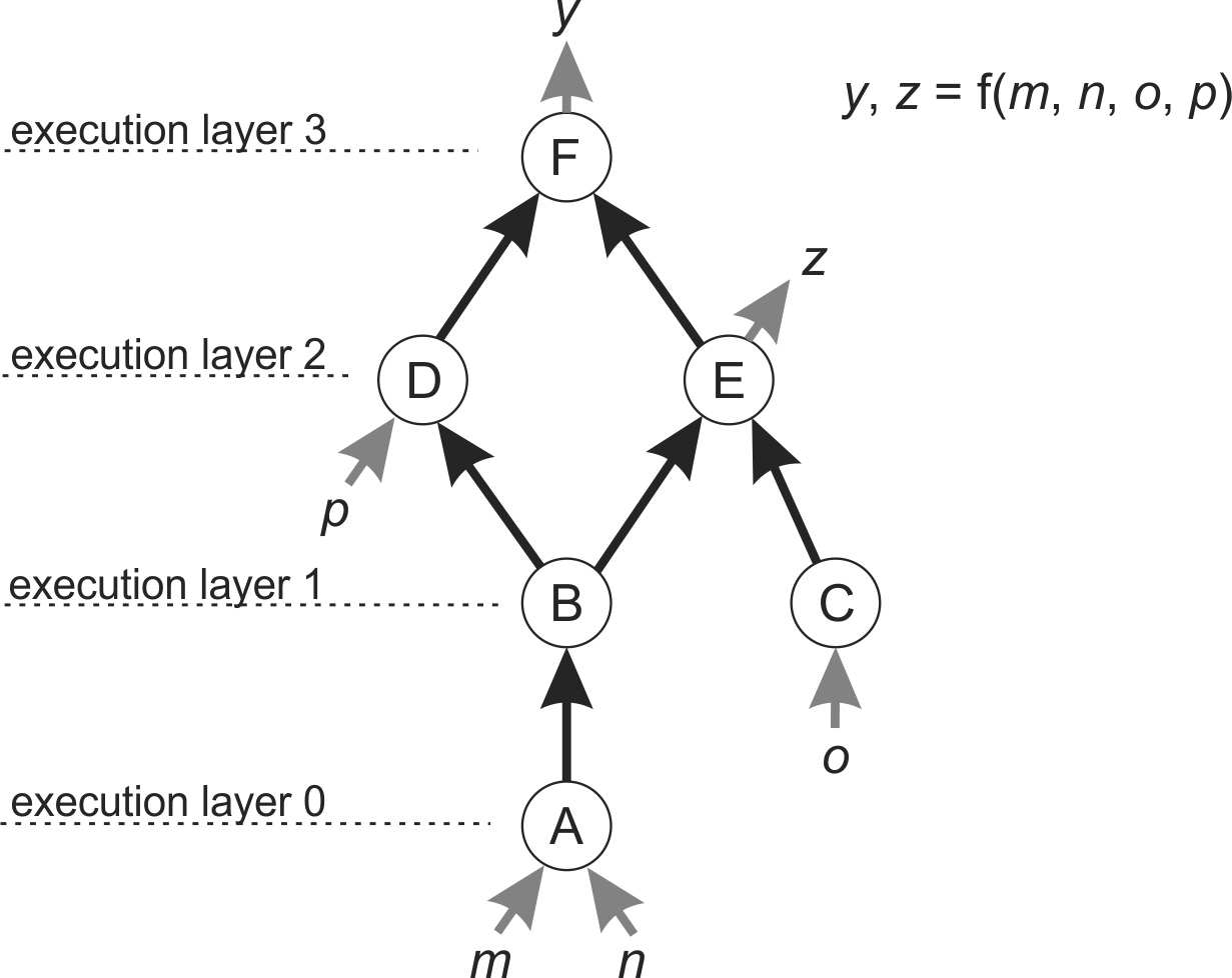
A graph with nodes A to F, inputs m to p and outputs y and z.
Many processes both man-made and in nature are cyclic. However a directed graph of functions must be acyclic if it is to be optimized: a cyclic graph will run forever.